
Introduction
Retrieval-Augmented Generation (RAG) is a powerful method that enhances the capabilities of language models by combining external information retrieval with natural language generation.
Normally, the interaction with a language model is simple and direct: A user asks a question → the AI model generates a response based purely on its internal training.
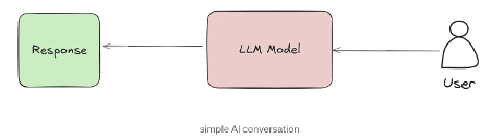
In this setup, the AI depends entirely on the knowledge it learned during its training phase. It cannot access new information or adapt to specific domains like medicine, law, or academic research without being retrained, which is costly and impractical.
This is where RAG comes in. Instead of relying only on what the model already knows, RAG introduces an important new step: retrieving relevant information from external documents in real time.
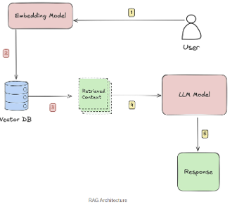
Here’s the big picture:
- First, an embedding model transforms documents into dense numerical representations known as vectors. These vectors capture the semantic meaning of the text — not just matching keywords, but understanding the relationships and ideas within the content.
- Next, these vectors are stored in a vector database, making it possible to perform similarity searches. When a user submits a query, the system can quickly retrieve the most relevant pieces of information based on meaning, not just words
This combination of vectorization and retrieval is what allows modern RAG systems to be so much more powerful, flexible, and accurate.
To understand how retrieval works, we first need to understand what these vectors are — and how an embedding model creates them from raw text.
What are Vector Embeddings
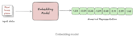
A vector is simply a list of numbers that represent certain properties of an object. When it comes to text, a good embedding model transforms a sentence, paragraph, or even an entire document into a high-dimensional vector that captures its meaning, not just the words it uses.
In this context, “high-dimensional” means that each vector isn’t just a handful of numbers — it can have hundreds or even thousands of dimensions. Each dimension encodes some subtle aspect of the sentence’s meaning, like topic, tone, or context. While we can’t easily visualize spaces beyond three dimensions, think of it this way: instead of plotting points on a simple 2D graph (X and Y) or even a 3D space (X, Y, and Z), embeddings exist in spaces with hundreds of invisible axes (e.g., 784 dimensions).
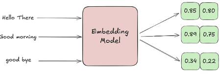
Imagine representing each sentence with just two numbers — like coordinates on a 2D map. Each number captures a hidden feature learned by the model, such as tone or topic.
Example Sentences and Their Embeddings:
Explanation:
- “Hello there” and “Good morning” have very close coordinates because they are both greetings — their meanings are similar.
- “Good bye” is farther away because, even though it’s still a polite phrase, it expresses ending rather than starting a conversation, so the meaning is different.
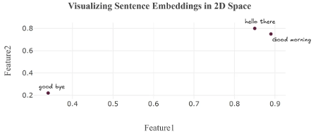
In this 2D space, each sentence is represented as a point based on its meaning. “Hello there” and “Good morning” appear close together because they are both greetings, while “Goodbye” is farther away, reflecting its different intent.
Embedding Models
There are many embedding models available today some general-purpose, others fine-tuned for specific tasks. To compare their performance, a popular benchmark is the MTEB (Massive Text Embedding Benchmark) leaderboard. Hosted by Hugging Face, it offers a wide range of benchmark results across various tasks. However, it’s important to approach it with some caution: many results are self-reported, and models that perform well in benchmarks don’t always translate to strong results in real-world applications.
Simple Example: How Different Embedding Models Create Different Vectors Here’s an example that demonstrates how different embedding models produce different vector representations of the same text:
from sentence_transformers import SentenceTransformer
import numpy as np
# Select two different embedding models from HuggingFace
models = {
"all-MiniLM-L6-v2": "Small general-purpose model (384D)",
"all-mpnet-base-v2": "Larger general-purpose model (768D)"
}
# Sample sentences to compare
sentences = [
"Remi Loves Pizza!",
"Ahmed loves modern cars"
]
# Compare embeddings from both models
for model_name, description in models.items():
print(f"\n=== {model_name} ===")
print(f"Description: {description}")
# Load model and generate embeddings
model = SentenceTransformer(model_name)
embeddings = model.encode(sentences)
# Show vector details for each sentence
for i, sentence in enumerate(sentences):
print(f"\nSentence {i+1}: '{sentence}'")
print(f"Vector shape: {embeddings[i].shape}")
print(f"First 5 values: {np.round(embeddings[i][:5], 4)}...")The output:
=== all-MiniLM-L6-v2 ===
Description: Small general-purpose model (384D)
Sentence 1: 'Remi Loves Pizza!'
Vector shape: (384,)
First 5 values: [-0.0545 0.012 -0.002 0.0215 -0.093 ]...
Sentence 2: 'Ahmed loves modern cars'
Vector shape: (384,)
First 5 values: [ 0.0438 0.1236 0.0049 0.0179 -0.0249]...
=== all-mpnet-base-v2 ===
Description: Larger general-purpose model (768D)
Sentence 1: 'Remi Loves Pizza!'
Vector shape: (768,)
First 5 values: [-0.0608 0.0307 -0.0257 0.0192 0.0719]...
Sentence 2: 'Ahmed loves modern cars'
Vector shape: (768,)
First 5 values: [-0.0462 0.0551 -0.0059 0.0316 -0.0381]...- Vector Shape: Each model produces embeddings with different sizes because they are built with different architectures. all-MiniLM-L6-v2: 384-dimensional vectors, While all-mpnet-base-v2: 768-dimensional vectors.
- First 5 Values: Even for the same sentence, the numeric values in the embeddings differ between models and This happens because:
- They are trained on different datasets.
- They use different model architectures.
- They optimize different trade-offs (speed vs. semantic richness).
While vectors differ numerically, good models preserve semantic relationships in their relative positioning — similar texts should have similar vectors within the same model’s space, even if absolute values differ across models.
let’s look at a real-world example.
We’ll take several sentences that all use the word “right”, but in completely different contexts — direction, legal entitlement, correctness, physical sides, and timing, Even though the same word appears in each sentence, the true meaning behind each usage is very different.
A good embedding model groups similar meanings together and keeps different meanings separate.
We’ll encode each sentence, measure how similar they are, and see whether the model captures their true meanings, not just shared words.
Load the model:
from sentence_transformers import SentenceTransformer
from sklearn.metrics.pairwise import cosine_similarity
import matplotlib.pyplot as plt
import seaborn as sns
# Load model
model = SentenceTransformer("all-mpnet-base-v2")Define sentences using the word “right” in different contexts.
# Original sentences and their similar counterparts
original_sentences = [
"Turn right at the traffic light", # Direction
"You have the right to remain silent", # Legal entitlement
"That answer is completely right", # Correctness
"The right side of the fabric is shiny", # Physical side
"Right after lunch, we'll leave" # Temporal (immediately)
]
similar_sentences = [
"Take a 90-degree turn at the intersection", # Direction (similar meaning)
"The law entitles you to not speak", # Legal (similar meaning)
"The solution is 100% correct", # Correctness (similar meaning)
"The front face of the material glows", # Physical side (similar meaning)
"Immediately following the meal, we depart" # Temporal (similar meaning)
]
all_sentences = original_sentences + similar_sentencesConvert each sentence into a high-dimensional vector representation embeddings = model.encode(sentences).
Calculate and display the similarity between each pair of sentences in a readable table. (We’ll explain how these similarity metrics work in detail later.)
# Labels for plotting
labels = [
"Direction", "Legal", "Correct", "Physical", "Temporal",
"Direction (sim)", "Legal (sim)", "Correct (sim)", "Physical (sim)", "Temporal (sim)"
]
# Generate embeddings
embeddings = model.encode(all_sentences)
# Create similarity matrix
similarity_matrix = cosine_similarity(embeddings)
# Print similarity between each original and its similar version
print("\nSimilarity between original and similar sentences:\n")
for i in range(5):
sim = cosine_similarity([embeddings[i]], [embeddings[i+5]])[0][0]
print(f"{labels[i]} vs {labels[i+5]}: {sim:.2f}")
# Full heatmap for all comparisons
plt.figure(figsize=(10,8))
sns.heatmap(similarity_matrix, annot=True, fmt=".2f", cmap="coolwarm",
xticklabels=labels, yticklabels=labels)
plt.title("Cosine Similarity between Original and Similar Sentences")
plt.xticks(rotation=45, ha='right')
plt.yticks(rotation=0)
plt.tight_layout()
plt.show()The output:
Similarity between original and similar sentences:
Direction vs Direction (sim): 0.60
Legal vs Legal (sim): 0.66
Correct vs Correct (sim): 0.56
Physical vs Physical (sim): 0.54
Temporal vs Temporal (sim): 0.64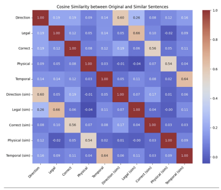
Even though the sentences use different phrases, the model correctly matches sentences based on their meaning. In the heatmap and scores, each original sentence is most similar to its matching sentence — like “Direction” and “Direction (sim)” scoring 0.60.
While we’ve created meaningful embeddings, but that’s just the first step. With these embeddings represented as vectors, we can apply mathematical operations to explore how closely related two sentences are.
This is where similarity metrics come in — tools like dot product and cosine similarity help us measure how close two sentences really are in meaning.
How We Compare Sentence Embeddings
In machine learning, similarity metrics are mathematical tools that measure how “alike” two things are — whether they’re words, images, or even entire documents.
Understanding these metrics is crucial because the way we measure similarity directly affects the quality of tasks like:
- Searching for related documents
- Grouping similar conversations
- Detecting duplicates
- Recommending content
There are many ways to measure the distance or similarity between vectors, but We’ll focus on the most commonly used ones for NLP tasks.
1 Cosine Similarity
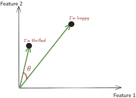
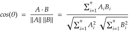
Cosine similarity measures the angle between two vectors, not their actual length. Think of two arrows pointing in space — cosine similarity checks if they are pointing in the same direction, even if one arrow is longer than the other.
Let’s see a simple example of how we can calculate cosine similarity, both manually and using a popular Python library.
import math
from sklearn.metrics.pairwise import cosine_similarity
import numpy as np
# Example vectors
A = [1, 2] #can represent a sentenec like I'm happy
B = [2, 3] #can represent a sentenec like I'm thrilled
# Manual calculation
dot = A[0]*B[0] + A[1]*B[1]
mag_A = math.sqrt(A[0]**2 + A[1]**2)
mag_B = math.sqrt(B[0]**2 + B[1]**2)
cosine_manual = dot / (mag_A * mag_B)
print(f"Manual Cosine Similarity: {cosine_manual:.3f}")
# Using sklearn
cosine_lib = cosine_similarity([A], [B])[0][0]
print(f"Sklearn Cosine Similarity: {cosine_lib:.3f}")Both the manual calculation and the library function give the same result: 0.992.
- A value close to 1 means the two vectors (and thus the two sentences) are very similar.
- If the value were closer to 0, it would mean they are unrelated.
- A value near -1 would mean they are opposite in meaning.
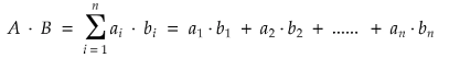
2 Dot Product
The dot product is one of the simplest ways to measure how two vectors are related. It’s a basic mathematical operation that multiplies two vectors together to give a single number, So when working with text embeddings, the dot product tells us how much two sentences “point” in the same direction.

- If the two vectors point the same way, the dot product is large and positive.
- If they are unrelated, the dot product is small.
- If they point in opposite directions, the dot product is negative.
The dot product is not normalized — so its value can be any real number, depending on the size (magnitude) of the vectors.
(This is different from cosine similarity, which is always between [-1,1])
import numpy as np
# Example vectors
A = [1, 2]
B = [2, 3]
# Manual calculation
dot_manual = A[0]*B[0] + A[1]*B[1]
print(f"Manual Dot Product: {dot_manual}")
# Using numpy
dot_np = np.dot(A, B)
print(f"Numpy Dot Product: {dot_np}")
#Result = 8Since our dot product is positive and fairly large, it tells us that the two vectors (and thus the two sentences they represent) are similar.
NOTE: Dot product is fast to compute and very efficient, which is why it’s often used inside models like attention mechanisms.
3 Euclidean Distance
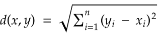
Another popular way to measure similarity (or rather, dissimilarity) between two vectors is the Euclidean distance, It measures the length of a line segment connecting these two points.
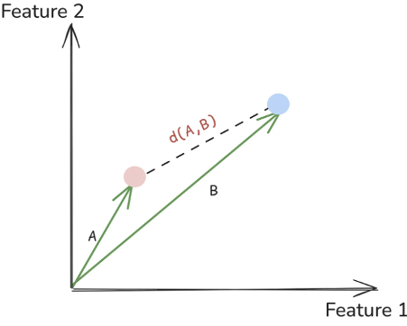
Unlike cosine similarity or dot product, Euclidean distance always measures how far apart vectors are so smaller distance means more similarity, and larger distance means less similarity.
import numpy as np
# Example vectors
A = [1, 2]
B = [4, 6]
# Manual calculation
diff_x = A[0] - B[0]
diff_y = A[1] - B[1]
euclidean_manual = np.sqrt(diff_x**2 + diff_y**2)
print(f"Manual Euclidean Distance: {euclidean_manual}")
# Using numpy
euclidean_np = np.linalg.norm(np.array(A) - np.array(B))
print(f"Numpy Euclidean Distance: {euclidean_np}")
# Result = 5.0Euclidean distance is simple and easy to understand, But when we move into very high-dimensional spaces (like 768 dimensions in sentence embeddings), it doesn’t work as well. In such spaces, distances between points start to feel very similar — this is called the curse of dimensionality. That’s why in NLP tasks, we often prefer cosine similarity instead.
Choosing the Right Similarity Metric
Picking the right similarity metric is crucial for getting the best results from your embeddings. The general rule is simple: use the same type of metric that was used when training your embedding model.
For example:
- If your model (like all-MiniLM-L6-v2) was trained with cosine similarity, you should also use cosine similarity in your system.
- If the model was trained with Euclidean distance, you should stick with Euclidean distance when comparing vectors.
Using the same metric ensures that the structure and relationships captured during training are preserved during retrieval or analysis.
Conclusion
In this article, we explored how vector search improves retrieval by comparing embeddings using similarity measures like cosine similarity, dot product, and Euclidean distance. We also discussed how choosing the right embedding model and metric is critical for optimizing RAG systems. Understanding these fundamentals is key to building more accurate and intelligent retrieval pipelines.